Hazard rate

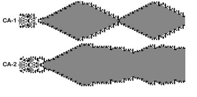
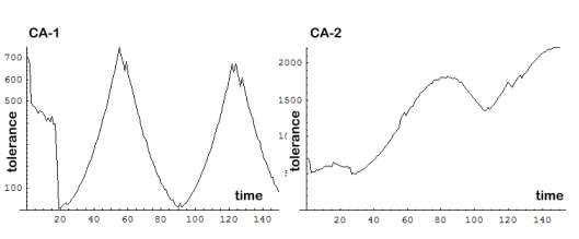
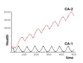
The present experiment is continuation  of the flip-flop experiment where the CA oscillated between two states, resource accumulation and output. Since it did not accumulate tolerance its health deteriorated. Health may be maintained by adding a tolerance accumulator to the system. The proliferon consists of a stem CA-0, CA-1 and CA-2.  CA-2 accumulates tolerance which he gets from CA-1.

delivery[2, 1, k, 2] ;
delivery[2, 2, k, 2] ;
If[ p[1,prev] > p[1,now], set rule[250]]; Min[++k, 40], else [set rule[600]]

The  CA  starts as isolated processes  (rule = 600). At time = 20 the demand starts rising.  When demand rises, CA-1 and CA-2  switch  between rules 600 and 250. When production{previous] > production[now]  the CA  apply rule-600 and raise  k, . When production{previous] <  production[now]  the CA  apply rule-250. At k = 40  they starts declining. Since CA-2 gets tolerance from CA-1 it declines less.

Both CA output tolerance (resources) and their velocities accelerate and decelerate. CA-2 [mean velocity] > CA-1[mean velocity]. On the average CA-2 accumulates tolerance faster than CA-1.

The health curves are similar  to the tolerance curves, since tolerance accumulation dominates the health equation.

Hazard rate

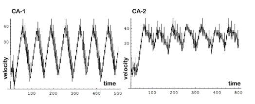
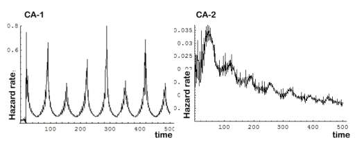
Hazard rate is a good measure of the  robustness of a CA. It is used by demographers to describe populations where it is known as force of mortality. Given a function f   its hazard rate is f’ / f   (derivative[f] / f ).   Here f is tolerance,  f’ is velocity, and hazard rate = v / tolerance.

The hazard rate of CA-1 oscillates. When CA-1 accumulates tolerance its hazard rate declines and during output it rises again. The hazard rate of CA-2 also oscillates, however since it accumulates tolerance the overall hazard declines.

 

---

delivery: [j, j-1, While[p[j-1] > set point], 2]
Argument[1]: Activated CA.
Argument[2]: Activating CA.
Argument[3]: Delivery condition.
Argument[4]: Delivery amount.
p[j]:  daily production